Community detection

📬 Get the future posts directly in your inbox:

I’ve been playing around with visualizations for street networks, and as a way to practice and improve with the use of custom color palettes with matplotlib I decided to do an exercise to look for communities in a street network and plot them using a custom color palette. All the code is available in this GitHub repo.

Data

The first step was to download the street network, for this I used OSMnx, and project it to the coordinate system to be able to plot the streets.

G_drive = ox.graph_from_place(
				'Guadalajara, Mexico',
				network_type='drive', 
				simplify=True, 
				which_result=2)
G_drive = ox.project_graph(G_drive)

The next step is to have a copy of the streets network converted into an undirected graph, this is because we will apply the Louvain Modularity algorithm for community detection, and it only work with undirected graphs. To create the undirected network we used the following function.

def undirected_network(G):
    G_simple = nx.Graph()
    for i,j,data in G.edges(data=True):
        w = data['weight'] if 'weight' in data else 1.0
        if G_simple.has_edge(i,j):
            G_simple[i][j]['weight'] += w
        else:
            G_simple.add_edge(i,j,weight=w)
    return G_simple

Community Detection

Now that we have the streets network that will be used to generate the plot and its simplified version for the community detection, we are ready to apply the algorithm. For this case I’m working with Networkx and created a function that returns a dictionary with the nodes of the network as keys and the community where they belong as values.

def find_communities(G):
    start_time = time.time()
    partition = louvain.best_partition(G)
    part_dict = {}
    values = []
    for node in G.nodes():
        values.append(partition.get(node))
        part_dict.update({node:partition.get(node)})
    communities_louvain= max(values)+1
    end_time = time.time()
    mod_louvain = louvain.modularity(partition,G_simple)
    print('Communities found using the Louvain algorithm: {}
    			\nModularity: {} \nTime for finding the communities:
					{} s'.format(communities_louvain, mod_louvain,
					round((end_time-start_time),3)))
    return part_dic

After getting the communities, I set the community attribute of the nodes in the streets network.

Color

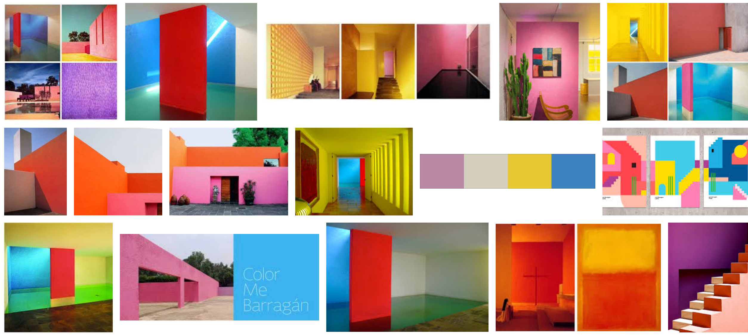
I started this experimentation because I wanted to use custom colors to generate a palette. I got inspired by Luis Barragán use of colors and decided to use his buildings to create the color palette.

#List of color
Color_barragan = ['#E1CF3F','#F47757','#FD4581','#97577C',
                 '#BDA7A9','#E1CF3F','#F47757','#FD4581',
                 '#e44623','#e45a6a','#c9d3e6','#7d513d',
                 '#e65949','#d6b240','#382a29','#d8d4c9',
                 '#e4cc34','#ccb42c','#bc8ca4','#3c84c4',
                 '#dd4d3d','#52172f','#63494a','#e2d5d3',
                 '#f7abcc','#e085a1','#943d39','#2d1d19']
#Create the color map
Barragan = mpcol.ListedColormap(Color_barragan, name='Barragan')

After creating the color map, I assigned each color to one community, so I can use it to plot the network with each node colored by the community they belong to.

com = [x[1] for x in G_drive.nodes(data='community')]
norm = mpcol.Normalize(vmin=min(com), vmax=max(com), clip=True)
mapper = cm.ScalarMappable(norm=norm, cmap=Barragan)
nc=[mapper.to_rgba(x) for x in com]

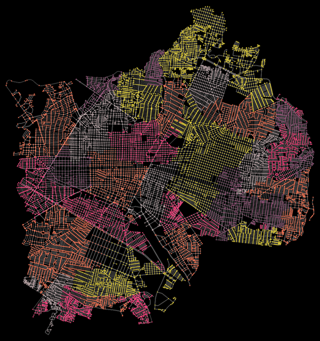
Plot

The final step was to plot the network using the newly mapped colors, and again OSMnx came to the rescue with the plotting functionality.

save = False
name = 'Guadalajara'
fig, ax = ox.plot_graph(G_drive, bgcolor='black', node_color=nc, node_size=8.5, node_zorder=3, node_alpha=1, edge_linewidth=0.25, edge_color='white',edge_alpha=1,fig_height=20,close=True, show=True, save=save, filename=name, file_format='png')

💬 Join the conversation:

Keep to conversation with a comment or reach out in my social networks.