The City That Never Sleeps
📬 Get the future posts directly in your inbox:
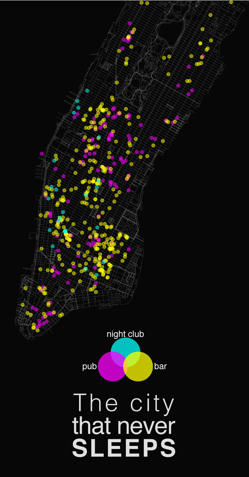
Today I found this data visualization by Shawn Allen, shared by Aaron Penne, and thought about doing something similar as an exercise for data manipulation and plotting. So I decided to do a plot about the bars, pubs, and night clubs in Manhattan. For the visualization that used python with some libraries, to create the dataset I used OSMnx to download the points of interest and store them into a GeoDataFrame in GeoPandas, that latter was combined with the Manhattan walking network to produce the visualization with Matplotlib.
Code
The first step after importing the basic libraries to work with was to get the data. For this step I had some data already downloaded, the walking graph and the shape of the city, for the points of interest I download and cleaned them.
def load_data(name):
    area = gpd.read_file('Data/{}/{}_shape/'.format(name, name))
    area = ox.project_gdf(area, to_crs=crs_osm)
    geometry = area.unary_union
    pois = ox.pois_from_polygon(geometry, amenities=['bar','pub','nightclub'])
    pois = ox.project_gdf(pois, to_crs=crs_osm)

    for item in ['way', 'relation']:
        pois.loc[pois.element_type==item, 'geometry'] = \
            pois[pois.element_type==item]['geometry'].map(lambda x: x.centroid)

    pois['geometry_type'] = pois.geometry.map(type)

    s=pois['geometry']
    pois['x'] = s.apply(lambda p: p.x)
    pois['y'] = s.apply(lambda p: p.y)

    dat_fin = gpd.sjoin(pois, area, op = 'within')
    pois = dat_fin

    G = ox.load_graphml('{}/{}_walk.graphml'.format(name,name))
    G = ox.project_graph(G, to_crs=crs_osm)
    return G, pois
The previous function returns the graph and point of interest to be plotted. The next step is straight forward, plot the graph and on top of it the different points as scatter plots with different colors, in this case, Yellow, Magenta, and Cyan as if they were ink being printed with the CMYK color model.
def make_plot(G, pois):
    fig, ax = ox.plot_graph(G, node_color='#aaaaaa', node_size=0, show=False, close=True, fig_height=20, edge_linewidth=0.1, bgcolor='black',edge_color='#969494')
    ax.scatter(pois.loc[pois['amenity'] == 'pub']['x'],pois.loc[pois['amenity'] == 'pub']['y'], zorder=3, c='magenta', alpha=0.5, marker='o',s=30)
    ax.scatter(pois.loc[pois['amenity'] == 'bar']['x'],pois.loc[pois['amenity'] == 'bar']['y'], zorder=3, c='yellow', alpha=0.5, marker='o',s=30)
    ax.scatter(pois.loc[pois['amenity'] == 'nightclub']['x'],pois.loc[pois['amenity'] == 'nightclub']['y'], zorder=3, c='cyan', alpha=0.5, marker='o',s=30)
    suptitle_font = {'family':'DejaVu Sans', 'fontsize':45, 'fontweight':'normal', 'y':0.15, 'color':'white'}
    fig.canvas.draw()
    fig.savefig('imgs/{}_nightlife.png'.format(name),transparent=True, dpi=300)
    fig
And here is the final result after adding the text and legend in illustrator:
📬 Get the blog posts directly in your inbox:
💬 Join the conversation:
Keep to conversation with a comment or reach out in my social networks.